The data that we analyzed in the book chapter actually come from a pretest-posttest design in which individuals were randomly assigned to a treatment or a control condition, and they were measured with experience sampling prior to treatment, and afterwards again. Hence, we have intensive longitudinal data from two episodes (i.e., pre-intervention and post-intervention), from two groups of individuals (i.e., treated and non-treated).

Data structure

If we have intensive longitudinal data that were obtained at multiple waves, for instance in a pretest-posttest design, or in a measurement-burst design, it is preferable to have the waves represented in wide format, while the repeated measures within a wave are represented in long format.

Below we see an example of what the original data structure may be: It contains a separate column for each separate variables that was measured within an individual, including:

ID: a variable that indicates which person a row belongs to
T: a variable that indicates time (in this case since the beginning of the first day of the study)
X and Y: two momentary measurements
P: a baseline covariate that is measured prior to each episode of intensive longitudinal measurements
E: a variable that indicates which episode (or wave) an observation belongs to
G: a variable that indicates what group a person belongs to (this does not vary within a person)

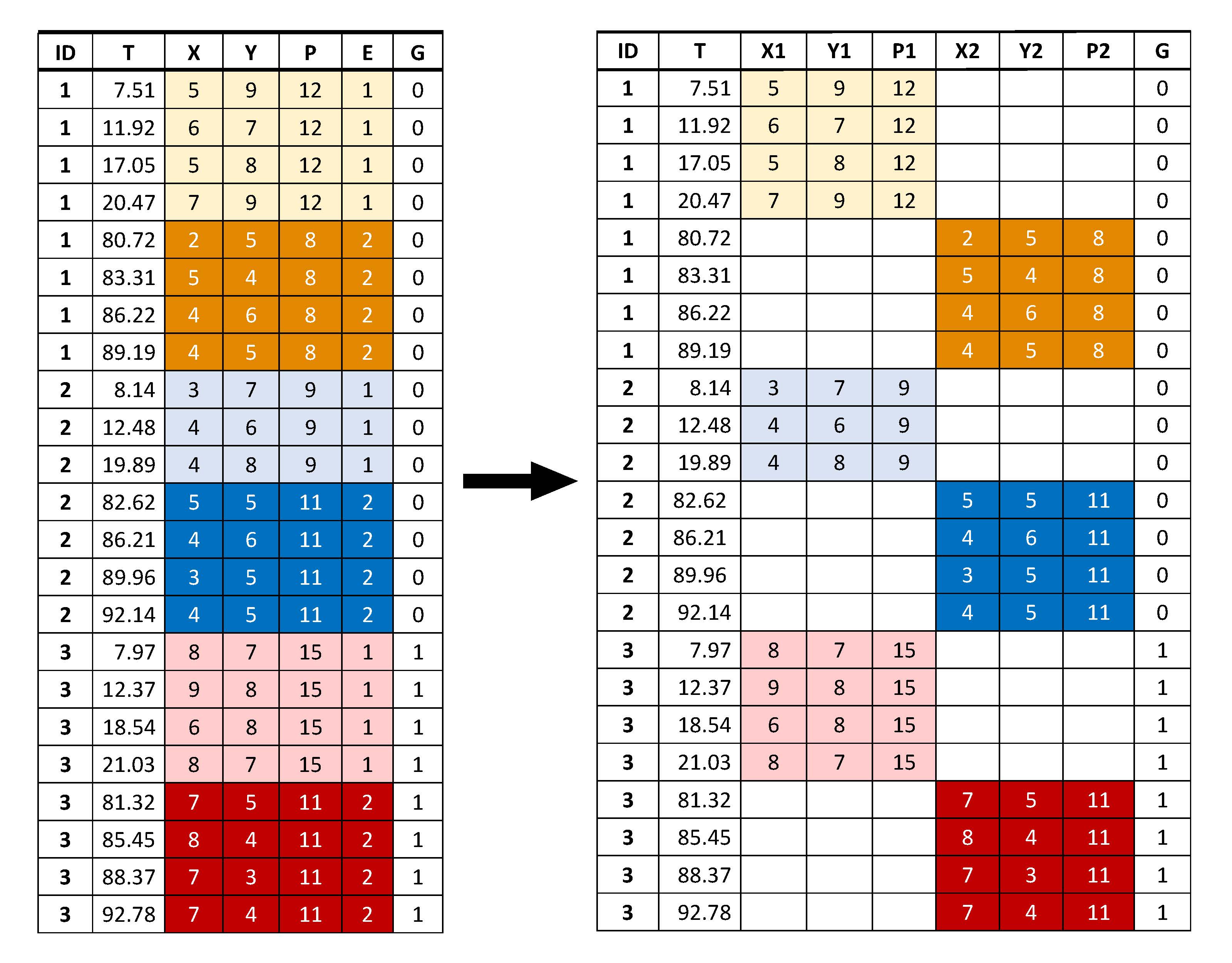
These data are restructured such that the measurements that vary within a person (either from moment to moment, such as X and Y, or from one wave to the next, such as P) are represented by different columns for different episodes. As a consequence, these newly created variables will contain many missings.

The advantage of this approach is that the variables will now be decomposed into a within-person and a between-person component per episode. This allows us to investigate changes in the means of individuals, but also in their autoregressive, cross-regressive and (residual) variances from one wave to another.

Model

We are interested in whether there are changes in specific aspects of the intensive longitudinal measurements due to treatment. Specifically, our focus is on changes in the individuals':

average tendency to experience negative affect, that is, the mean on negative affect: \(\Delta y_i^{(b)}= y2_i^{(b)} - y1_{i}^{(b)}\)
inertia of negative affect, that is, the autoregressive parameter for negative affect: \(\Delta \phi_{i} =\phi_{2i} - \phi_{1i}\)
sensitivity of negative affect to unpleasantness events, that is, the cross-regression from unpleasantness of events to negative effect: \(\Delta \beta_{i} =\beta_{2i} - \beta_{1i}\)
sensitivity of negative affect to other factors, that is, the residual variance of negative affect: \(\Delta \phi_{i} =\phi_{2i} - \phi_{1i}\)
average level of unpleasant events experienced, that is, the mean on unpleasantness of events: \(\Delta \psi_{i} =\psi_{2i} - \psi_{1i}\)

We are interested in whether these changes are a result of time, and to what extent they are the results of treatment. Furthermore, to make it possible to make sensible comparisons, we should also consider whether there were initial differences between the two treatment groups prior to treatment.

T investigate all these aspects, we regress all the random effects on the dummy variable \(G_i\), which equals 1 for the treated and 0 for the untreated. Hence, at the within level for we have:

\[\begin{align*} y1_{it}^{(w)} &= \phi_{1i} y1_{it-1}^{(w)} + \beta_{1i} x1_{it}^{(w)} + \zeta_{xit}\\ y2_{it}^{(w)} &= \phi_{2i} y2_{it-1}^{(w)} + \beta_{2i} x2_{it}^{(w)} + \zeta_{xit} \end{align*}\]

where the first equation is for the variable containing the data from the first episode (prior to treatment), and the second equation is for the variable containing the data for the second episode (after treatment). Note that the autoregressions and the cross-regressions are not constrained to be the same across these episodes.

At the between level we now have

\[\begin{align*} y1_{i}^{(b)} &= \gamma_{00} + \gamma_{01} G_i + u_{0i}\\\ \phi_{1i} &=\gamma_{10} + \gamma_{11} G_i + u_{1i}\\ \beta_{1i} &= \gamma_{20} + \gamma_{21} G_i + u_{2i}\\ log(\psi_{1i})&= \gamma_{30} + \gamma_{31} G_i + u_{3i}\\ x1_{it}^{(b)} &= \gamma_{40} + \gamma_{41} G_i + u_{4i}\\ \\ \Delta y_{i}^{(b)} = y2_{i}^{(b)}-y1_i^{(b)}&=\gamma_{50} + \gamma_{51} G_i + u_{5i} \\ \Delta \phi_{i} = \phi_{2i} - \phi_{1i}&=\gamma_{60} + \gamma_{61} G_i + u_{6i}\\ \Delta \beta_{i} = \beta_{2i} - \beta_{1i} &= \gamma_{70} + \gamma_{71} G_i + u_{7i}\\ \Delta log(\psi_{i})= log(\psi_{2i}) - log(\psi_{1i})&=\gamma_{80} + \gamma_{81} G_i + u_{8i}\\ \Delta x_{it}^{(b)} = x2_{it}^{(b)}-x1_{it}^{(b)}&=\gamma_{90} + \gamma_{91} G_i + u_{9i} \end{align*}\]

where the first set of five regressions equations are for the random effects associated with episode 1, while the second set of five regression equations are for the changes in the random effects from episode 1 to episode 2.

Hence

the regression parameters \(\gamma_{01}\) to \(\gamma_{41}\) indicate whether there are initial differences between the two groups
the regression parameters \(\gamma_{51}\) to \(\gamma_{91}\) indicate whether there are group differences in the changes of the random effects (i.e., a treatment effect)
the intercepts \(\gamma_{50}\) to \(\gamma_{90}\) indicate whether there is a change in the random effects for the no-treatment group (i.e., a time effect)

Input

To specify this model in Mplus, we have to indicate which variable we specify the VARIABLE command as:

  VARIABLE:
  NAMES       =   ID prepost TimeHours U2P PA NA PEx NEx
                  pa_pre na_pre U2P_pre PEx_pre NEx_pre
                  pa_post na_post U2P_post PEx_post NEx_post
                  ham_pre ham_post group;
  CLUSTER     =   ID;
  USEVAR      =   na_pre na_post group ue_pre ue_post;
  BETWEEN     =   group;
  LAGGED      =   na_pre(1) na_post(1);
  TINTERVAL   =   TimeHours(1);
  MISSING     =   ALL(-999);

that is, we make use of the two variables that form the outcome variable of interest during each episode (for which we also create lagged versions so we can include autoregression), the grouping variable (with information about the treatment group each person belongs to; this is a between level variable), and the two variables that serve as the time-varying predictor during each episode.

The DEFINE command is used to create the predictor variable for each episode, by multiplying an observed variable from the data set by minus 1 (as we also did in all the other analyses):

  DEFINE:     ue_pre = -1*U2P_pre;
              ue_post = -1*U2P_post;

The ANALYSIS command is also similar to what we had before:

  ANALYSIS:   TYPE = TWOLEVEL RANDOM;
                ESTIMATOR = BAYES;
              PROC = 2;
              BITER = (3000);
              BSEED = 8386;
              THIN = 5;

The MODEL command contains two parts again. The within part is:

  MODEL:
      %WITHIN%
      phi_pre | na_pre ON na_pre&1;
      beta_pre | na_pre ON ue_pre;
      psi_pre | na_pre;
      phi_post | na_post ON na_post&1;
      beta_post | na_post ON ue_post;
      psi_post | na_post;
      ue_pre WITH ue_post@0;

where the first three lines are for the first episode, and the second set of three lines is for the second episode. The last line is to ensure that Mplus does not try to estimate the covariance of the two exogenous variables; not that these variables will never be both observed within the same occasion, because the observation took either part during the first episode, meaning that ue_pre will be observed and ue_post will be missing, of the observation took place during the second episode, meaning that ue_post is observed and ue_pre is missing.

Note that this is also true for na_pre and na_post; however, we do not have to constrain the residuals of these variables to be uncorrelated, or to be uncorrelated with ue_pre and ue_post, as we have defined the residuals to come from a individual specific distribution (using the | notation); such random (residual) variances are by definition for components that are not correlated with other components.

At the between level we want to:

regress the random effects associated with the first episode on the grouping variable \(G_i\), to ensure there were no initial differences between the randomly created groups
regress the change in each of the random effects between the two episodes on the grouping variable \(G_i\), to investigate the effect of treatment.

The latter is however not possible, as Mplus does not allow us to regress the change between two random effects on another variable. However, we can accomplish the same by regressing the random effect of the second episode on the random effect at the first episode and fixing the regression coefficient to one. For instance, for the change in individual mean of negative affect we have:

\[\Delta y_i^{(b)} = y2_i^{(b)} - y1_i^{(b)} = \gamma_{50} + \gamma_{51} G_i + u_{5i}\]

which can be rewritten as

\[y2_i^{(b)} = \gamma_{50} + \gamma_{51} G_i + y1_i^{(b)} + u_{5i}\]

Hence, the between level is now defined as

      %BETWEEN%
      na_pre ue_pre phi_pre beta_pre psi_pre ON group;
      na_post ON na_pre@1 group;
      ue_post ON ue_pre@1 group;
      phi_post ON phi_pre@1 group;
      beta_post ON beta_pre@1 group;
      psi_post ON psi_pre@1 group;

Output

The output for this analysis is can be found here.

We obtain the following parameter estimates for this model:

MODEL RESULTS

                                Posterior  One-Tailed         95% C.I.
                    Estimate       S.D.      P-Value   Lower 2.5%  Upper 2.5%  Significance

Within Level

 UE_PRE   WITH
    UE_POST            0.000       0.000      1.000       0.000       0.000

 Variances
    UE_PRE             2.838       0.053      0.000       2.734       2.942      *
    UE_POST            2.253       0.042      0.000       2.174       2.342      *

Between Level

 PHI_POST   ON
    PHI_PRE            1.000       0.000      0.000       1.000       1.000

 BETA_POST  ON
    BETA_PRE           1.000       0.000      0.000       1.000       1.000

 PSI_POST   ON
    PSI_PRE            1.000       0.000      0.000       1.000       1.000

 PHI_PRE    ON
    GROUP              0.079       0.041      0.030      -0.005       0.159

 BETA_PRE   ON
    GROUP             -0.013       0.015      0.195      -0.042       0.016

 PSI_PRE    ON
    GROUP              0.010       0.170      0.472      -0.312       0.351

 PHI_POST   ON
    GROUP             -0.132       0.060      0.018      -0.247      -0.007      *

 BETA_POST  ON
    GROUP              0.018       0.019      0.165      -0.019       0.054

 PSI_POST   ON
    GROUP             -0.240       0.172      0.083      -0.574       0.116

 NA_PRE     ON
    GROUP             -0.028       0.126      0.415      -0.278       0.219

 UE_PRE     ON
    GROUP              0.095       0.106      0.195      -0.112       0.300

 NA_POST    ON
    NA_PRE             1.000       0.000      0.000       1.000       1.000
    GROUP             -0.286       0.098      0.002      -0.480      -0.096      *

 UE_POST    ON
    UE_PRE             1.000       0.000      0.000       1.000       1.000
    GROUP             -0.264       0.081      0.001      -0.421      -0.106      *

 UE_POST  WITH
    NA_POST            0.079       0.025      0.000       0.038       0.133      *

 Intercepts
    NA_PRE             2.025       0.088      0.000       1.847       2.198      *
    NA_POST            0.023       0.067      0.364      -0.107       0.157
    UE_PRE            -1.301       0.073      0.000      -1.445      -1.162      *
    UE_POST           -0.085       0.056      0.066      -0.196       0.029
    PHI_PRE            0.451       0.030      0.000       0.392       0.508      *
    BETA_PRE           0.116       0.011      0.000       0.096       0.137      *
    PSI_PRE           -1.163       0.118      0.000      -1.394      -0.931      *
    PHI_POST          -0.044       0.042      0.148      -0.130       0.037
    BETA_POST         -0.012       0.013      0.173      -0.037       0.013
    PSI_POST          -0.267       0.120      0.016      -0.508      -0.029      *

 Residual Variances
    NA_PRE             0.468       0.068      0.000       0.359       0.623      *
    NA_POST            0.229       0.043      0.000       0.161       0.325      *
    UE_PRE             0.276       0.042      0.000       0.209       0.371      *
    UE_POST            0.091       0.026      0.000       0.051       0.149      *
    PHI_PRE            0.034       0.006      0.000       0.023       0.049      *
    BETA_PRE           0.004       0.001      0.000       0.002       0.006      *
    PSI_PRE            0.841       0.116      0.000       0.650       1.107      *
    PHI_POST           0.061       0.014      0.000       0.039       0.093      *
    BETA_POST          0.004       0.001      0.000       0.002       0.007      *
    PSI_POST           0.767       0.124      0.000       0.569       1.066      *

Note that we are not explicitly modeling unpleasantness of events (it is merely included as a predictor in this model); hence Mplus estimates its variance for the two episodes (represented as two separate variables in the data file) at the within level and these can be considered average within-person variances.

Furthermore, we see that none of the episode 1 random effects are predictable from the grouping variable; this indicates that there are no meaningful differences between the randomly created groups.

There are three random effects whose change depends on the treatment group:

na_post, after regressing on na_pre and fixing the regression coefficient to 1, has group as a negative predictor (i.e., \(\gamma_{51}= -0.286\)), meaning that the average negative affect people report has decreased (on average) after treatment
ue_post, after regressing on ue_pre and fixing the regression coefficient to 1, has group as a negative predictor (i.e., \(\gamma_{91} = -0.264\)), meaning that the average level of unpleasantness of events that people report has decreased (on average) after treatment
phi_post, after regressing on phi_pre and fixing the regression coefficient to 1, has group as a negative predictor (i.e., \(\gamma_{61} = -0.132\)), meaning that the carry-over or inertia of negative affect has decreased after treatment

When considering the intercepts of the random effects of the second episode, there is only one that deviates from zero, indicating a time effect (rather than a treatment effect): It is for intercept of psi_post (which is actually the log of the residual variance of negative affect), which is: \(\gamma_{80}=-0.267\). This implies there is a reduction in the residual variance of negative affect over time, which could mean that over time individual become less sensitive to unmeasured factors.

Pretest-posttest analyses

Data structure

Model

Input

Output